

ここでは、はてなブログの「今週のはてなブログランキング」で2022年1月から12月までに紹介されたブログのタイトルを分析してみて、その結果を紹介しています。
目的としては、人気記事のタイトルにどんな言葉が使用されているのか知りたかったためです。SEO的な調査のためという事ではないです。
この記事の対象
前準備
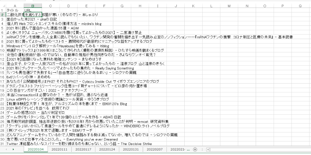
該当の2022年の1月~12月までのランキングのタイトルを予め、エクセルに保存しておきます。はてなブログはスクレイピングが禁止のようなのでお気をつけ下さい。
今回は手動でコピペして以下のような形で保存していきました。
行ったこと(プログラムの流れ)
- 任意のエクセルファイルの読込み
- 形態素解析(Mecab)
- 単語ごとに出現回数をカウント
- 出現回数の多い順にソート
- 上位30件の単語と出現回数を表示
- WordCloudの作成
- 2-gramのTree Map作成
流れとしてはざっくりと上記になります。ここでは外部ライブラリを使用しているので、それぞれpipでインストールしておく必要があります。
pip install squarify wordcloudプログラム
import MeCab
import matplotlib.pyplot as plt
from wordcloud import WordCloud
import numpy as np
import openpyxl
import japanize_matplotlib
from squarify import plot as tree_map
import plotly.graph_objects as go
import networkx as nx

FONT_PATH = r"C:\hoge\AppData\Local\Programs\Python\Python311\Lib\site-packages\matplotlib\mpl-data\fonts\ttf\ipaexg.ttf"
#1---Excelファイルからタイトルを読み込む
wb = openpyxl.load_workbook('read.xlsx')
titles = []
for sheet_name in wb.sheetnames:
    ws = wb[sheet_name]
    for row in ws.iter_rows(min_row=2, min_col=1, max_col=1, values_only=True):
        title = row[0]
        if title:
            titles.append(title)

#2---形態素解析を行う
m = MeCab.Tagger("C:\Program Files\MeCab\dic\mecab-ipadic-neologd")
words = []
for title in titles:
    node = m.parseToNode(title)
    while node:
        word = node.surface
        pos = node.feature.split(',')[0]
        if pos in ['名詞', '形容詞', '動詞'] and word != " ":
            words.append(word)
        node = node.next

#3---単語ごとに出現回数をカウントする
counts = {}
for word in words:
    if word in counts:
        counts[word] += 1
    else:
        counts[word] = 1

#4---出現回数が多い順にソートする
sorted_counts = sorted(counts.items(), key=lambda x: x[1], reverse=True)

#5---上位30件の単語と出現回数を表示する
for i, (word, count) in enumerate(sorted_counts[:30]):
    print(f"{i+1}: {word} - {count}")

#6---ワードクラウドを作成する
wordcloud = WordCloud(font_path=FONT_PATH,background_color='white', width=800, height=600).generate_from_frequencies(counts)
plt.imshow(wordcloud)
plt.axis('off')
plt.savefig('test1-1.png')

plt.clf()
#7---2-gramごとに出現回数をカウントする
n_gram_counts = {}
for i in range(len(words)-1):
    word_pair = (words[i], words[i+1])
    if word_pair in n_gram_counts:
        n_gram_counts[word_pair] += 1
    else:
        n_gram_counts[word_pair] = 1

#8---出現回数が多い順にソートする
sorted_n_gram_counts = sorted(n_gram_counts.items(), key=lambda x: x[1], reverse=True)

#9---上位20件の2-gramと出現回数を表示する
for i, (word_pair, count) in enumerate(sorted_n_gram_counts[:20]):
    print(f"{i+1}: {' '.join(word_pair)} - {count}")

#10---2-gramのtree mapを作成する
labels = [' '.join(word_pair) for word_pair, count in sorted_n_gram_counts[:20]]
values = [count for word_pair, count in sorted_n_gram_counts[:20]]
norm_values = [value / sum(values) for value in values]
color = [plt.cm.Spectral(x) for x in np.linspace(0, 1, len(labels))]
tree_map(norm_values, label=labels, color=color, alpha=.7)
plt.axis('off')
plt.savefig('test1-2.png')

plt.clf()
#11---単語同士の関係をnetworkxのグラフに追加する
G = nx.Graph()
max_word_count = 1 # 表示する単語の最大出現回数
for i in range(len(words)-1):
    word1 = words[i]
    word2 = words[i+1]
    if word1 in counts and counts[word1] > max_word_count:
        continue
    if word2 in counts and counts[word2] > max_word_count:
        continue
    if G.has_edge(word1, word2):
        G[word1][word2]['weight'] += 1
    else:
        G.add_edge(word1, word2, weight=1)

#12---グラフを描画する
pos = nx.spring_layout(G, k=0.9)
edge_labels = {(u, v): d['weight'] for u, v, d in G.edges(data=True)}
node_sizes = [counts[word] * 10 for word in G.nodes()]
nx.draw_networkx_nodes(G, pos, node_size=node_sizes, node_color='lightgray')
nx.draw_networkx_edges(G, pos, edge_color='lightgray', width=[d['weight']/50 for u, v, d in G.edges(data=True)])
nx.draw_networkx_labels(G, pos, font_size=8, font_family='IPAexGothic', font_weight='bold')
nx.draw_networkx_edge_labels(G, pos, edge_labels=edge_labels, font_size=8, font_family='IPAexGothic')
plt.axis('off')
plt.savefig('test1-3.png')
頻出単語
#3---単語ごとに出現回数をカウントする
counts = {}
for word in words:
if word in counts:
counts[word] += 1
else:
counts[word] = 1
#4---出現回数が多い順にソートする
sorted_counts = sorted(counts.items(), key=lambda x: x[1], reverse=True)
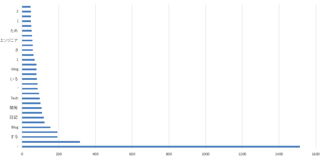
#5---上位30件の単語と出現回数を表示する
for i, (word, count) in enumerate(sorted_counts[:30]):
print(f"{i+1}: {word} - {count}")3、4、5の部分で解析とソートを行った上でグラフ化してみました。記号があったり一文字のものがあったりであまりちゃんと上手く形態素解析ができていない事がわかります。
【結果】
WordCloud
#6---ワードクラウドを作成する
wordcloud = WordCloud(font_path=FONT_PATH,background_color='white', width=800, height=600).generate_from_frequencies(counts)
plt.imshow(wordcloud)
plt.axis('off')
plt.savefig('test1-1.png')
6の部分では、WordCloudを作成しています。ここでは日本語が文字化けしないように予め「import japanize_matplotlib」をインストールしておく必要があります。
【結果】

N-gram tree Map
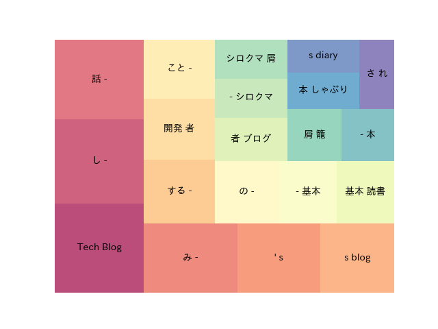
#9---上位20件の2-gramと出現回数を表示する
for i, (word_pair, count) in enumerate(sorted_n_gram_counts[:20]):
    print(f"{i+1}: {' '.join(word_pair)} - {count}")

#10---2-gramのtree mapを作成する
labels = [' '.join(word_pair) for word_pair, count in sorted_n_gram_counts[:20]]
values = [count for word_pair, count in sorted_n_gram_counts[:20]]
norm_values = [value / sum(values) for value in values]
color = [plt.cm.Spectral(x) for x in np.linspace(0, 1, len(labels))]
tree_map(norm_values, label=labels, color=color, alpha=.7)
plt.axis('off')
plt.savefig('test1-2.png')
9、10の部分ではN-gramについての処理を行っています。N-gramの方も上手く行ってないです。最初に単語の抽出方法が悪いと残念な結果になることが身にしみています。笑
詳しいN-gramについては以下をご参照下さい。
【結果】
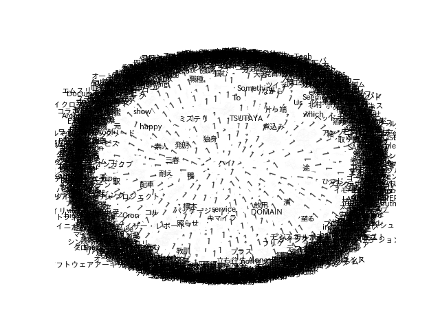
ネットワーク図
#11---単語同士の関係をnetworkxのグラフに追加する
G = nx.Graph()
max_word_count = 1 # 表示する単語の最大出現回数
for i in range(len(words)-1):
    word1 = words[i]
    word2 = words[i+1]
    if word1 in counts and counts[word1] > max_word_count:
        continue
    if word2 in counts and counts[word2] > max_word_count:
        continue
    if G.has_edge(word1, word2):
        G[word1][word2]['weight'] += 1
    else:
        G.add_edge(word1, word2, weight=1)

#12---グラフを描画する
pos = nx.spring_layout(G, k=0.9)
edge_labels = {(u, v): d['weight'] for u, v, d in G.edges(data=True)}
node_sizes = [counts[word] * 10 for word in G.nodes()]
nx.draw_networkx_nodes(G, pos, node_size=node_sizes, node_color='lightgray')
nx.draw_networkx_edges(G, pos, edge_color='lightgray', width=[d['weight']/50 for u, v, d in G.edges(data=True)])
nx.draw_networkx_labels(G, pos, font_size=8, font_family='IPAexGothic', font_weight='bold')
nx.draw_networkx_edge_labels(G, pos, edge_labels=edge_labels, font_size=8, font_family='IPAexGothic')
plt.axis('off')
plt.savefig('test1-3.png')
ネットワークを作成してみました。しかし、上手くパラメータを調整できず、汚い感じになってしまいました。
【結果】
まとめ
可視化してみましたが、上手くいかないものですね。去年の人気記事のタイトルには「開発」「Blog」などが頻繁に出てくるようでした。
WordCloudを見るとBlogやサービス、方法など出てきています。技術ブログに関係しそうなキーワードが多い印象を受けます。
まだまだ改善の余地があるので、次は記号は無視した場合で挑戦してみたいと思います。